California Wildfires Have Fat Tails Part One: The Statistics

The recent, devastating wildfires in Southern California highlight the importance of anticipating, and planning for, rare but extremely damaging natural events.  The impact of Hurricane Helene on parts of Appalachia is another example of low-probability, high-consequence natural disasters that can be devastating to human and natural communities.

Wildfires and windstorms occur regularly but exceptionally large wildfires and hurricanes are rare. Yet both types of events occur often enough that there are data from which we can describe and understand their statistical properties.  I believe that this understanding can help people prepare for these events and manage their impacts.

This blog addresses these topics, focusing on wildfires that occur in California.  Part one of the blog addresses the statistical properties of these wildfires and those of other natural disasters.  Part two speaks to how people can use those properties to prepare for, and to some degree manage, these events and their consequences.  

Further, low-probability, high consequence circumstances can be devastating in other parts of our society, especially to financial institutions that rely on financial leverage (i.e., lots of debt, relatively little equity) in their capital structures.  For example, the principal business of commercial banks is to lend money to people and businesses and make a profit doing so.  Under normal circumstances, most borrowers repay their loans and banks are profitable.  Rarely, though, banks encounter credit crises in which many borrowers default and banks become unprofitable.  Some even fail.

The statistical properties of credit losses at banks have similarities to losses suffered from wildfires, so I will draw on my experience as a quantitative risk manager at financial institutions to support my conclusions about wildfires in California.

Be forewarned, this part of the blog is a relatively deep dive into statistics.  I begin with a description of the Normal distribution and its properties.

The Normal Distribution

The Normal, or Gaussian, statistical distribution is the one with which most people are familiar since it describes many common features of our lives, including the birth weight of babies, the height of adult males in the United States, diastolic blood pressure for those males, shoe sizes of those men, and scores on the ACT college entrance test, among other things.

The Normal distribution is symmetrical and bell-shaped around its central point (Figure 1).  That central point is, simultaneously, the mean (average), median (midpoint) and mode (most common value) of that distribution.  Accordingly, 50% of the values in the distribution fall below the mean and 50% above the mean (hence the median equals the mean).

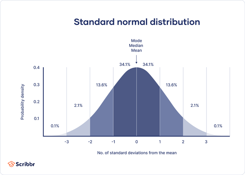
Figure 1.  The Standard Normal Distribution. 

Source: Scribbor.

Several other properties of the Normal distribution follow from these characteristics.  First, the symmetry means that the left and right sides are mirror images.  Second, the variance of the distribution, which is the sum of squared deviations from the mean, and the standard deviation of the distribution, which is the square root of the variance, both represent the variability of the distribution.  In the Standard Normal distribution, the mean (µ) equals zero (0) and both the variance (σ2) and the standard deviation (σ) equal one (1) (see Figure 1). 

The symmetry and bell shape of the Normal distribution dictate that most of the observations in the distribution are concentrated near the mean and those observations are equally distributed on either side of the mean (Figure 1).  Specifically, 34.1 percent of all observations in the distribution lie between the mean and one standard deviation to the right.  Between the mean and one standard deviation to the left is another 34.1 percent of all observations in the distribution.  Thus, 68.2 percent of all observations lie between µ plus σ and µ minus σ.  Further, µ +/- 2σ equals 95.4 percent of all observations and 99.7 percent of all observations fall with µ +/- 3σ (Figure 1).

The “Tails” of a Statistical Distribution

The edges or ends of a statistical distribution, representing observations significantly greater or smaller than the mean, are called “tails.”  Since there are few such extreme values in the Standard Normal distribution, its tails are termed “thin.”  A thin-tailed distribution is one with few outliers and a concentration of data near the mean.

However, many of the risks that people and institutions face do not conform to the Normal distribution.  One example is credit losses incurred by banks when they lend money to people and businesses.

In Figure 2, I plot the distribution of annual loan losses (charge-offs[1]) in Citibank’s commercial lending portfolios from 1974 to 2023.

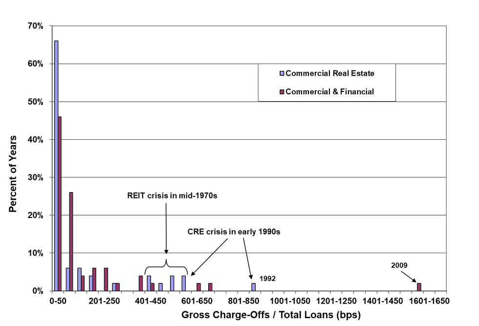
Figure 2.  Distribution of Losses in Citibank N.A.’s U.S. Commercial Loan Portfolios, 1974 to 2023

Source: Citigroup Annual Reports

We see immediately that the pattern in Figure 2 is very different from the one in Figure 1.  Instead of being symmetrical around the center as in the Standard Normal distribution, loan losses have a highly skewed distribution.  Half or more of all years experienced 50 basis points (bps)[2] or fewer of loan losses and loan losses of 400 bps occurred in relatively few years.  These periods of exceptionally high losses occur in credit crises, periodic lending catastrophes that I explain in detail in my recent book, Credit Crises: The Role of Excess Capital (Stevenson, 2024).

This distribution has three defining characteristics that make it different from a Normal distribution:

1.      It is not symmetrical but is skewed with a long tail stretching out to the right.

2.      Small losses are very common and exceptionally large losses are both less common than the small ones but more common than would be expected if the distribution were Normal.

3.      The most frequent value is less than the average or mean value.

These characteristics define the distribution as “fat-tailed,” specifically a distribution in which extreme values occur more frequently than they do in a Normal distribution.

There are a number of advanced statistical metrics that evaluate whether or not a statistical distribution exhibits a fat tail and several “rules of thumb” that also determine “fat-tailedness” as well as two core measures of the shape of a distribution.  In this blog, I use these rules of thumb as they are likely to appeal to, and be understood by, the broadest array of readers.  I also use statistical measures of the shape of a frequency or probability distribution, including skewness and kurtosis.

Let’s begin with the first rule.  If the value at the 98th percentile of the distribution[3] is 5.6 times greater (or more) than the value at the 50th percentile (median), then the distribution is fat-tailed.  If the ratio of the 98th percentile to the 50th percentile is less than 5.6, then the distribution is thin-tailed.

The second rule of thumb holds that, if the ratio of the 98th percentile to the mode is greater than, or equal to, 16, the distribution is fat-tailed.  If this ratio is less than 16, the distribution is thin-tailed.

In the case of charge-offs in Citibank’s commercial loan portfolios, the median value of charge-offs is 43 bps and the value at the 98th percentile is 666 bps (Figure 2).  The ratio of these two numbers is 15.5, making the distribution of loan losses fat-tailed.

With respect to the second rule of thumb, the mode of the distribution of loan losses is zero (0).  Unfortunately, this means that the ratio of the 98th percentile to the 50th percentile is undefined, since the denominator is zero.  Thus, this rule cannot provide insight into the fat-tailedness of Citibank’s loan losses.

Skewness 

In statistics, “skewness” is the degree of asymmetry in a probability or frequency distribution. When data points are not distributed symmetrically to the left and right sides of the median, the distribution is skewed. A Normal distribution exhibits zero skewness because of its symmetry.

Distributions can be positive and right-skewed, or negative and left-skewed. A right-skewed or positive distribution means its tail is more pronounced on the right side than on the left. Most of the values in the distribution occur to the left of the mean value. The most extreme values are on the right side.  

In a negative or left-skewed distribution, the tail is more pronounced on the left side than on the right. Most values are found to the right side of the mean in negative skewness. As such, the most extreme values are found further to the left.

The statistical skewness of the loan loss data shown in Figure 32 is 3.7.  The positive sign on this result confirms that the distribution is right-skewed and the magnitude of 3.7 confirms that the distribution deviates significantly from a Normal distribution in which statistical skewness equals zero (0).

Kurtosis

Kurtosis is a statistical measurement that reveals how dispersed are the data in a distribution and how likely the distribution is to have outliers[4].  Kurtosis captures three elements of the shape of that distribution:

• Tailedness: how often outliers occur and how far the tails extend.

• Peakedness: how peaked is the distribution.

• Heavy-tailedness: how heavy are the distribution’s tails.

  
  

The kurtosis of a Normal distribution is three (3) which is the benchmark against which the kurtosis of another distribution is compared.  For example, the kurtosis of Citibank’s loss losses is 18.3 which means that this distribution is more peaked and fat-tailed than a Normal distribution, both of which are evident in Figure 2.

In the second part of this blog, we will briefly explore what fat-tailedness means to the management of credit risk in bank portfolios to provide us insight into the management of wildfires in California.

So, let us now turn to the statistical properties of those California wildfires.

Wildfires in California

Wildfires are an important feature of the natural ecosystems in California and have been for millennia.  In fact, wildfires are critical force that has shaped those ecosystems, resulting in many natural adaptations to fire.  According to the California Department of Fish and Wildlife, “almost all of California’s diverse ecosystems are fire-dependent or fire-adapted”[5].

Fire-Dependent Ecosystems in California.  Fire-dependent ecosystems need wildfire to maintain appropriate function and health, while fire-adapted ecosystems have evolved to survive wildfire.[6]

Chaparral, for example, is a shrubby, sclerophyllous vegetation type that is common in middle elevations throughout much of California (Barro & Canard, 1991).  It is typically found on steep terrain and has great value in stabilizing those slopes, providing habitat for wildlife, and cycling nutrients. 

Chaparral is highly flammable and, when wildfires strike chaparral, they burn intensely often to the point in which the vegetative cover is destroyed.  Post-fire flooding and mudslides are possible due to the loss of vegetative cover to the soil.

Chaparral is the natural vegetation of some of the areas in California most densely inhabited by people, including Los Angeles and its suburbs.  As a result, these communities exist in an ecosystem that is not only adapted to fire but one that burns readily and intensely.  Damage to homes and other human structures can be significant, as occurred in the devastating Eaton and Palisades fires of early 2025.

CAL FIRE.  The California Department of Forestry and Fire Protection (CAL FIRE) is an organization within California state government dedicated to fire prevention, fire protection and stewardship in over 31 million acres of California’s privately-owned wildlands[7].  Preventing wildfires is a vital part of CAL FIRE’s mission as are pre-fire engineering of wildlands, management of vegetation, planning for fires and fire remediation, education, and law enforcement.  In addition, the Department provides varied emergency services in 36 of the State’s 58 counties via contracts with local governments.

CAL FIRE has multiple goals[8], including:

• Fire prevention: Reduce the risk of wildfires through forest health work, defensible space inspections, and controlled burns.

  
  

• Fire protection: Contain 95% of fires at 10 acres or less. 

  
  

• Natural resource management: Protect and manage California's natural resources, including watersheds, wildlife, and timber resources. 

  
  

• Emergency response: Respond to fires, floods, earthquakes, medical aid, and other disasters.

• Public safety: Increase public safety and decrease the risk to firefighters. 

  
  

• Environmental protection: Ensure the highest level of environmental protection. 

  
  

• Wildfire resilience: Restore forests lost to wildfires and improve wildlife and fisheries habitat. 

  
  

CAL FIRE also publishes data on individual wildfires that occurred between 2016 and 2024, including the name of the fire or fire complex, the county(ies) in which the fire took place, the date it started and the number of acres burned by the fire[9]. 

In Figure 3, I plot, by number of acres burned, the distribution of the sizes of the 2,459 wildfires that occurred in California in this period.

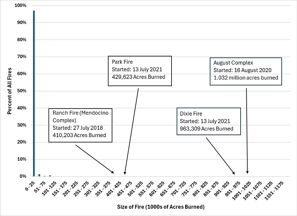
Figure 3.  Distribution of California Wildfires by Size of Fire, 2016 to 2024. 

Source: Cal Fire

We see immediately that wildfires in California do not follow a Normal distribution.  Instead, they fit one that has a strong positive skew to the right.  In addition, there is a dramatic peak in the number of fires in the smallest size category: fully 97.0% of these fires burned 25,000 acres or fewer. 

I hasten to add that a fire of 25,000 acres is not a small fire for those who have to fight it or to those who suffer from its consequences.  For example, the Eaton and Palisades fires of January 2025[10], that devasted Altadena, Pacific Palisades, Pasadena and Sierra Madre, each burned fewer than 25,000 acres (Eaton: 14,021 and Palisade: 23,707 acres).[11]  So, these fires were not the among the largest in terms of acres burned but they were among the largest in terms of people killed and homes and other structures destroyed.

The four largest wildfires that occurred in the 2016 to 2024 period burned more than 400,000 acres each, many times larger than the 4,401 acres burned in the average fire.  The median of the distribution in Figure 3 is 77 acres burned and the mode is 10 acres.  (The fact that the mean is different from the mode which is different from the median confirms our conclusion that this distribution is not a Normal one.)

The right-handed skew in Figure 3 is the most pronounced that we’ve seen in this blog. In fact, the statistical skewness for California wildfires is 19.3, much larger than the 3.7 for Citibank’s loan loss distribution (Figure 2).  In addition, the kurtosis of this distribution is 463.2, indicating that the distribution of wildfires is much more peaked and fat-tailed that a Normal one (Figure 3).

So wildfires in California have fat tails.  Is this result consistent with wildfires elsewhere and with other types of natural disasters?  Yes.  In fact, there is considerable evidence in the literature that the distribution of wildfires follow fat-tailed distributions elsewhere (Cui & Perera, 2008; Cumming 2001; Keeting & Handmer, 2013; Koh, 2023; Malamud et al., 1998).

Damages from other natural disasters also follow fat-tailed distributions.  For example, Conte and Kelly (2018) demonstrated that the distribution of damage resulting from tropical storms in the U.S., including hurricanes, is fat-tailed, partly as a result of the fat-tailed distribution of human populations in coastal cities.

Damages from floods in the United States also follow fat-tailed distributions (Cooke et al., 2014)[12].

Conclusion

The distribution of wildfires in California wildfires is right skewed and has a fat tail, as do wildfires all across the globe.  This result is consistent with the conclusion that natural catastrophes create fat-tailed distributions in terms of the areas and levels of damages incurred.  As a result, very large wildfires are rare but less rare than would be expected if the pattern of wildfires followed a Normal distribution.

The fact that wildfires do not conform to a Normal distribution has very important implications for how people plan for wildfires, how they fight wildfires, and how they protect themselves, and recover, from wildfires.  I address these points in the second half of this blog, again in the context of California wildfires.

References

Barro, S. C. & Conard, S. G.  (1991).  Fire effects in California chaparral systems: An overview.  Environment International 17: 135-149.  https://doi.org/10.1016/0160-4120(91)90096-9

Conte, M. N. & Kelly, D. L. (2018). An imperfect storm: Fat-tailed tropical cyclone damages, insurance and climate policy.  Journal of Environmental Economics and Management 92: 677-706.  https://doi.org/10.1016/j.jeem.2017.08.010

Cooke, R. M., Nieboer, & J. Misiewicz. (2014).  Fat-Tailed Distributions: Data, Diagnostics and Dependence.  Volume 1 (Mathematical Models and Methods in Reliability Set,1) Hoboken, NJ: John Wiley & Sons, Inc.  144 pp.

Cui, W. & Perera, A. H. (2008).  What do we know about fire size distribution, and why is this knowledge useful for forest management?  International Journal of Wildland Fire 17: 234-244.

Cumming, S. G. (2001).  A parametric model of the fire-size distribution.  Canadian Journal of Forest Research 31(8): 1297-1303.  https://doi.org/10.1139/x01-032

Keeting, A. & Handmer, J. (2013). Catastrophic fat tails and non-smooth damage functions-fire economics and climate change adaptation for public policy. In: González-Cabán, Armando, tech. coord. Proceedings of the fourth international symposium on fire economics, planning, and policy: climate change and wildfires. Gen. Tech. Rep. PSW-GTR-245 (English). Albany, CA: U.S. Department of Agriculture, Forest Service, Pacific Southwest Research Station: 147-151.

Koh, J. 2023.  Gradient boosting with extreme value theory for wildfire prediction.  Extremes 26: 273-299.  https://doi.org/10.1007/s10687-022-00454-6

Malamud, B. D, Morein, G. & Turcotte, D. L.  (1998). Forest fires: An example of self-organized critical behavior, Science 281(5384): 1840–1842.

Stevenson, B. G. (2024).  Credit Crises: The Role of Excess Capital.  Tampa, FL: Gatekeeper Press.  450 pp.

[1] When a bank determines that a borrower has defaulted on its loan, it recognizes the amount the borrower will not repay.  The bank charges this amount as a loss to loan income In its accounting system and classifies it as a “charge-off.”

[2] A basis point (bp) is 1/100 of a percent.  Fifty bps is 0.50 percent.

[3] A percentile is a grouping of observations in which the observations are arranged from smallest to largest (or by some other classification) and divided into 100 units, each representing one percent of those arranged observations.  In this example, the 98th percent includes all observations, arranged from smallest to largest, except those observations that represent the largest two percent.

[4] An outlier is a data point or observation in a data set that lies outside of the range of, and significantly different from, other observations in the dataset.

[5] https://wildlife.ca.gov/Science-Institute/Wildfire-Impacts.  Last accessed 18 February 2025.

[6]Ibid

[7] https://www.fire.ca.gov.  Last accessed 8 February 2025.

[8] Ibid.

[9] Damage resulting from a wildfire can be measured in a number of ways, including human deaths, destruction of buildings and other structures and number of acres burned.  In the data on wildfires published by CAL FIRE, only number of acres burned is shown for each fire.

[10] These two fires are not included in the data set of California wildfires analyzed in this blog since that data set includes fires that started between 2016 and 2024, inclusive, and considered 100 percent contained or nearly so.

[11] https://www.fire.ca.gov/incidents/2025.  Last accessed 17 February 2025.

[12] Also see https://www.reseources.org/ common-resources/flood-insurance-claims-a-fat-tail-getting-fatter/.  Last accessed 18 February 2025.